The idea is pretty simple: more athletic athletes are probably better at athletics than less athletic athletes. Still, it’s worth investigating any model, no matter how intuitive. Statistics also give us the benefit of determining just how much things matter, rather than the qualitative idea of “well, it probably matters.”

Before we get into the particulars, here are the different things I’ll be working with in this study:

Approximate Value – To fully investigate the impact of athleticism, it’s necessary to develop a method of assigning value to each player. As our study is intended to cover all positions, it isn’t possible to use production-based metrics, and games started aren’t necessarily a measure of value. All-Pro and Pro Bowl honors give an idea of what players are performing better, but it’s too discrete and only applies to a handful of players each year. We need something that can be applied to thousands of data points.

This is where Approximate Value comes in. Developed by Doug Drinen at Pro-Football-Reference.com, it’s a metric that gives us an integer result which represents a given player’s value for a full season. Now, AV is not perfect. I know that, and Doug knows that. This is what he wrote about it:

AV is not meant to be a be-all end-all metric. Football stat lines just do not come close to capturing all the contributions of a player the way they do in baseball and basketball. If one player is a 16 and another is a 14, we can’t be very confident that the 16AV player actually had a better season than the 14AV player. But I am pretty confident that the collection of all players with 16AV played better, as an entire group, than the collection of all players with 14AV. – Doug Drinen

The idea is that, given a large data set, Approximate Value will get things right in a broad way. With a sample size of thousands, any biases or issues with the formula wash out, leaving us with a rough idea of player value. It’s not a perfect solution, but it’s the only thing we have to conduct large, position-independent studies.

I will specifically refer to “AV3” – I’ve defined this as the sum of a given player’s three best Approximate Value seasons. This means we’re measuring peak performance. We also include the NFL betting statistics of bookmaker betting sites, as they have many data available. Others have conducted studies using the first four years of AV (i.e., the length of a rookie contract), and that’s also a valid way of expressing player value.

pSPARQ –SPARQ is a formula that measures a player’s athleticism. A higher SPARQ means a more athletic player. The specifics, inputs, etc. are all covered in other articles linked to on this site (like this one).

We then normalize pSPARQ by position. A nose tackle isn’t going to test as well as a wide receiver, so we need to somehow represent how athletic each player is by their positional average. This is possible by calculating the z-score (standard score), which is the number of standard deviations that a player’s score is above the given positional mean. Read about it on the wiki.

The idea is that we can use these standard scores and relate how athletic each player is by a single number. A 0 z-score means a player is an average NFL athlete. A z-score of 2.0 means a player is an exceptional athlete. A “3-sigma” athlete doesn’t happen very often – the NFL only has 4 current players meeting this spec.

(Those 4 players: J.J. Watt, Calvin Johnson, Evan Mathis, and Lane Johnson)

Statistical Significance – Rather than try to explain this concept, I’ll let Wikipedia do it. The main takeaway is that statistics are able to tell us the probability that a relationship exists between two variables. This all boils down to the p-value; if the p-value is 0.25, that means there is a 25% chance that the two variables are unrelated. “Significant” p-values often are smaller than 0.05, meaning there’s a  5% likelihood of no relationship (and by corollary, a 95% chance that there does exist a link). Any p-value less than 0.01 is very strong.

Weighted Least Squares Regression (WLS) – We’re working with a pretty large data set, and the scatter plot ends up being too dense to really comprehend.  The other issue is that there are a lot of zero-AVs in this data set, i.e., there are a number of players who never contributed significantly to the NFL.  This makes a scatter plot even more difficult visually because we can’t see that there are 100 scatter points stacked on top of each other at a given point.

In this kind of set, it’s common to use a weighted least squares regression, operating on the mean of the data at a list of discrete points. For our purposes, this means we would see the average AV3 of all players with a 0.2 z-score, the average AV3 of all players with a 0.3 z-score, and so on.

By operating on the mean of the data, we do not change the test for statistical significance. WLS will produce the same linear regression and strength of relationship while making it visually digestible.

With the preamble over, we can actually start regressing things.

First, let’s look at every player in the database drafted from 1999-2012. This means that we’re including 9,560 data points, drafted and undrafted. It’s probably not the best way to do things, but it’s just a starting point.

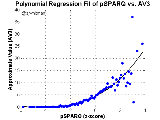
This isn’t an entirely surprising result. Undrafted players tend to be less athletic, and they just don’t succeed very often.

Note that the end of the spectrum shows data points between a z-score of 2.0 and 4.0. These look like “messy” points to the eye – there’s less of a straightforward pattern and quite a bit of scatter. This is because there are only a handful of players above 3 sigma, so averaging the data doesn’t have the smoothing effect it has in the middle of the graph, where it’s averaging hundreds of players per z-score. The scatter at the end looks odd, but we just don’t have much data there.

I won’t even bother with the statistics for the above regression as it doesn’t reflect the hypothesis we want to test. It’s probably a more relevant question to ask how this study would look if it only looked at drafted players.

I should note at this point that I am not be adjusting for draft position. This is because draft position is not causally prior to athleticism, meaning: players don’t become more athletic because they’re drafted high. They’re often drafted high due to athleticism.

We can address at a later point the relative value of athletes in different rounds, but that’s a different hypothesis. What I’m looking at in this piece is a macro-level study on if “Combine athleticism” matters. We already know it does if considering the entire group of NFL prospects. Does it matter if we restrict the sample to only the 250+ who get drafted each spring?

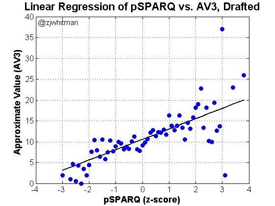
This looks promising, but more important is the p-value, which R reports as “< 2e-16.” This value is approximately zero, and there’s thus no chance that the relationship is just randomness. There is a statistically significant relationship between pSPARQ and Approximate Value. Yes, Combine events are able to measure the kind of athleticism that translates to NFL success.

I did some rolling averages over the end of the data to provide a little stability. Again, there are very few points from 2.0-4.0 on the x-axis, and the amount of scatter is deceptive. The following plot shows what it looks like with a little smoothing:

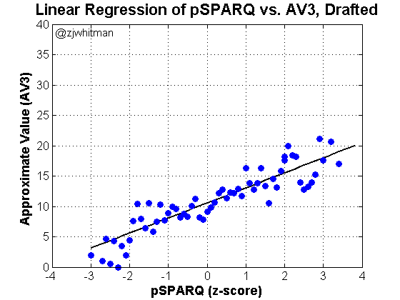
This is only intended to show that the data isn’t as messy as it appears. The regression is essentially the same as the first.

Note that this regression does not say that Player A with a 0 z-score is going to produce less AV than Player B with a 2.0 z-score. What it says it that a sufficiently large Group A of players that have a 0 z-score is going to produce less than those from Group B with a 2.0 z-score.

Remember that this is a starting point. It’s the most obvious regression to start with because it’s the largest. There are other, smaller studies that could be done at the positional level or with respect to draft position; however, this is a good start, and shows us that the test results we’ll see in Indianapolis do have some level of relevance.