UPDATE 4/20: The SPARQ table now includes most players with pro days occurring prior to March 20th. The image is a much higher-resolution than was used previously. Note that the “Comb.” column refers to those who were invited to the NFL Combine in February. Any numbers that are underlined and italicized comes from junior day data via Tony Wiltshire

Note that the “Percentile” and “z-score” columns refer to the NFL positional averages and not to the draft positional averages. This means that a 0.0 z-score and 50.0 percentile would represent a player who rates as a league-average NFL athlete at the position. The average NFL player is pretty athletic, so this designation is not at all a poor result.

Disclaimer: pSPARQ is not perfect and will not yield a perfect representation of any player’s athletic profile. It is meant to give us an idea of where a given player stands athletically relative to his peers. If you have any questions about the particulars, I posted an FAQ: https://3sigmaathlete.com/faq/.

Click on the images to make them readable.

All above the 50th percentile (i.e., above-average):

All below the 50th percentile:

–ZW

UPDATE 4/20: The SPARQ table now includes most players with pro days occurring prior to March 20th. The image is a much higher-resolution than was used previously. Note that the “Comb.” column refers to those who were invited to the NFL Combine in February. Any numbers that are underlined and italicized comes from junior day data via Tony Wiltshire.

Note that the “Percentile” and “z-score” columns refer to the NFL positional averages and not to the draft positional averages. This means that a 0.0 z-score and 50.0 percentile would represent a player who rates as a league-average NFL athlete at the position. The average NFL player is pretty athletic, so this designation is not at all a poor result.

Disclaimer: pSPARQ is not perfect and will not yield a perfect representation of any player’s athletic profile. It is meant to give us an idea of where a given player stands athletically relative to his peers. If you have any questions about the particulars, I posted an FAQ: https://3sigmaathlete.com/faq/.

Click on the images to make them readable.

All above the 50th percentile (i.e., above-average):

UPDATE 4/20: The SPARQ table now includes most players with pro days occurring prior to March 20th. The image is a much higher resolution than was used previously. Note that the “Comb.” column refers to those who were invited to the NFL Combine in February. Any numbers that are underlined and italicized comes from junior day data via Tony Wiltshire.

Note that the “Percentile” and “z-score” columns refer to the NFL positional averages and not to the draft positional averages. This means that a 0.0 z-score and 50.0 percentile would represent a player who rates as a league-average NFL athlete at the position. The average NFL player is pretty athletic, so this designation is not at all a poor result.

Disclaimer: pSPARQ is not perfect and will not yield a perfect representation of any player’s athletic profile. It is meant to give us an idea of where a given player stands athletically relative to his peers. If you have any questions about the particulars, I posted an FAQ: https://3sigmaathlete.com/faq/.

Click on the images to make them readable.

All above the 50th percentile (i.e., above-average):

All below the 50th percentile:

UPDATE 4/20: The SPARQ table now includes most players with pro days occurring prior to March 20th. The image is a much higher resolution than was used previously. Note that the “Comb.” column refers to those who were invited to the NFL Combine in February. Any numbers that are underlined and italicized comes from junior day data via https://www.bookmakers.eu/sports/american-football/.

Note that the “Percentile” and “z-score” columns refer to the NFL positional averages and not to the draft positional averages. This means that a 0.0 z-score and 50.0 percentile would represent a player who rates as a league-average NFL athlete at the position. The average NFL player is pretty athletic, so this designation is not at all a poor result.

Disclaimer: pSPARQ is not perfect and will not yield a perfect representation of any player’s athletic profile. It is meant to give us an idea of where a given player stands athletically relative to his peers. If you have any questions about the particulars, I posted an FAQ: https://3sigmaathlete.com/faq/.

Click on the images to make them readable.

All above the 50th percentile (i.e., above-average):

UPDATE 4/20: The SPARQ table now includes most players with pro days occurring prior to March 20th. The image is a much higher-resolution than was used previously. Note that the “Comb.” column refers to those who were invited to the NFL Combine in February. Any numbers that are underlined and italicized comes from junior day data via Tony Wiltshire.

Disclaimer: pSPARQ is not perfect and will not yield a perfect representation of any player’s athletic profile. It is meant to give us an idea of where a given player stands athletically relative to his peers. If you have any questions about the particulars, I posted an FAQ: https://3sigmaathlete.com/faq/.

Click on the images to make them readable.

All above the 50th percentile (i.e., above-average):

All below the 50th percentile:

Draft analytics aren’t necessarily about athleticism or SPARQ; the idea is to use data in a way that maximizes the use of draft capital. Before we discuss the specific model used here, it’s important to lay out the tools we’ll use in the analysis.

Approximate Value – Approximate Value is used to empirically measure player production. It’s not a perfect stat and won’t perfectly capture behavior at each position, but it functions well given a “large-enough” data set. As before, I’ll specifically use AV3, the sum of a given player’s best 3 seasons by Approximate Value. For a more detailed description of the stat, I’ll refer you to an earlier piece I wrote on the subject.

Bounds – This model includes all players drafted from 1999-2012. The information from 2013 and 2014 is potentially useful, but will not be utilized here as I hesitate to judge a player without 3 seasons of performance. Including the most recent draft classes would also mean comparing the career starts of the 2013/2014 prospects vs. the career peaks of players drafted in the mid-2000s and before.

ExpectedAV3 – Using the 99-12 player set, it’s possible to develop the average AV3 of players drafted in each round by position. This means we know what kind of AV3 is produced by a 5^th-round running back, 3^rd-round corner, and so on. To ensure as little bias as possible, ExpectedAV3 has been normalized by position.

Hit Rate – I’ve arbitrarily defined a “hit” as a player who generates an AV in the top 30% of all drafted players from the same position group. This gives us a metric which lends a bit more context than simply looking at raw Approximate Value stats. Note that I’ve used AV1, AV3, and AV5 in determination of hit rate. This means that a player can qualify with one exceptional year, three very good years, or five good-but-less-than-great years.

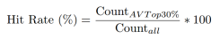
The 30% requirement for Hit Rate is arbitrary, but it serves us well for this purpose. The trends for each position from round-to-round are what we care about, and they’re fairly stable regardless of the benchmark value used to define a hit. 30% is also convenient as most successful NFL players fall in the top 30% of draftees at their position.

Positional ExpectedAV3 Curves

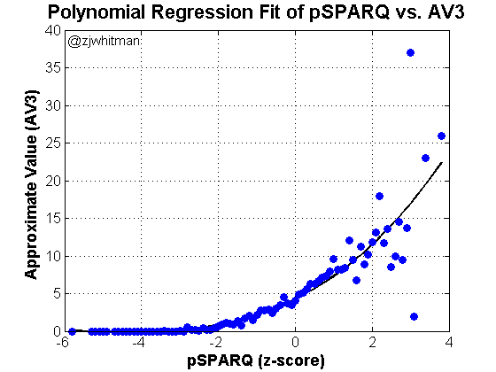
The most logical first step is to simply examine how a position varies with ExpectedAV3 by round. Note that the statistic is normalized such that an ExpectedAV3 equal to 1 is equivalent to the average player drafted at the position. This means that a player with ExpectedAV3 = 2 has produced double the average AV for the given position.

The following plot shows a typical ExpectedAV3 curve. Note that I’ve split up Round 1 into two sections – picks 1-16 are located at “1” on the x-axis and picks 17-32 are located at “1.5.”

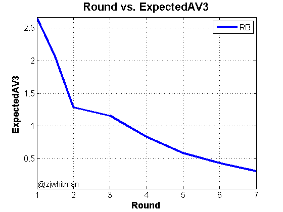
The most interesting part of the ExpectedAV3 plots is where the plateaus and drop-offs occur. With the above plot, we can see that there isn’t a huge difference between a running back drafted in the 2^nd and 3^rd round, but that group is much less productive than 1^st-rounders and much more productive than 4^th-rounders.

It’s still difficult to parse what exactly it means without relating it to other positions. Sure, we see a steep drop-off in production after the early rounds, but that’s not new information. It’s necessary to add context, and just stacking each position group in the same plot makes it too messy to discern much of anything.

MarginalAV3 Plots

To generate a plot that’s more visually digestible, I’ll use MarginalAV3, calculated by the following formula.

MarginalAV3 relates the average positional production for each round with the overall average. In simple terms, positions which produce more than expected in a particular round will have a positive value of MarginalAV3, and positions which are inefficient will have a negative MarginalAV3.

The following bar plots show the efficiency of each position group at each round.

Marginal Offensive Plots

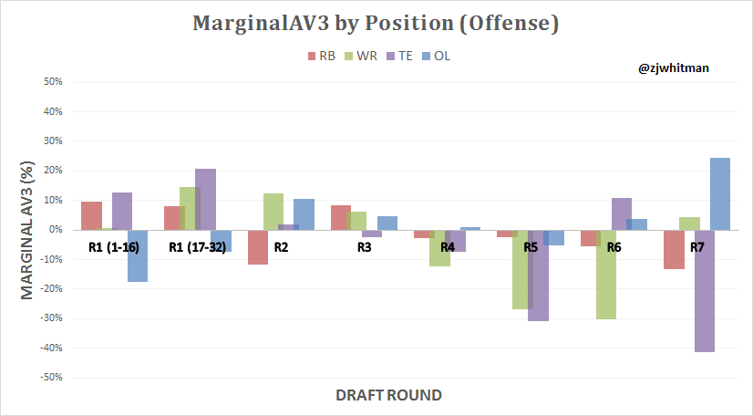
I would note that the sample size for tight ends is lower than that of other positions, so I’d take the large swings of rounds 5-7 with a grain of salt. The general trend is that the early rounds are where most relative tight end value is obtained, and there aren’t many tight ends drafted after the fourth round who yield much value.

There’s a clear trend overall that offensive picks struggle from the 4^th-6^th rounds. The second round produces the most positive offensive value on average.

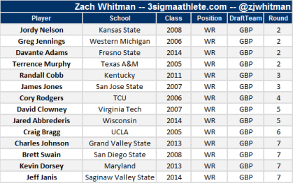
It’s apparent that wide receivers are a particularly terrible value pick in the 4^th-6^th rounds, but tend to produce surplus value in the 2^nd, 3^rd, and 7^th rounds. In Ted Thompson’s time as the general manager in Green Bay, he’s drafted 14 receivers. 10 of the 14 have come in surplus rounds, with only four being selected in the negative value rounds. Note that only one of the receivers from the negative value group was drafted after Thompson’s first three years as Green Bay GM.

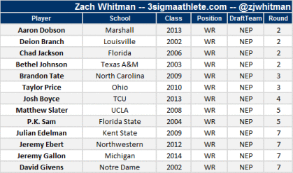
In Bill Belichick’s 15 New England drafts, he’s selected 10 of his 13 receivers in positive MarginalAV3 rounds, as shown below. While New England isn’t regarded as a wide receiver factory like Green Bay, they are more analytically-focused than most NFL franchises. It’s thus interesting to see how their draft strategy does or doesn’t conform to the data presented here.

The splits for the Patriots and Packers aren’t due to a league-wide shortage of receivers drafted in the negative value region. The 4^th-6^th average about the same number of WR picks as observed in the 2^nd and 3^rd rounds.

Marginal Defensive Plots

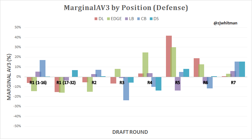
This plot is a bit more striking. We see that the biggest misses in early rounds are on EDGE players (and DL to a lesser extent). This isn’t saying that the great pass rushers aren’t found in the first round; the point is that teams aren’t good at evaluating EDGE players. DL and EDGE are less efficient markets than RB and WR; teams miss early more on the DL/EDGE than they do at any other position.

Hit Rate Plots

It’s important to understand context here. It’s not a perfect strategy to only select defensive linemen in the 5^th round; though this may historically be the most efficient round for the position, there still isn’t a great shot of getting a significant contributor. The hit rate at all positions in late rounds is low, and this data should be used in conjunction with the marginal plots.

The following plots show the hit rate of players drafted at each position in each round. As noted earlier, hit rate refers to all players who produced in the top 30% of their position according to AV criteria.

On Offense

Star tight ends are frequently drafted early. It typically requires a very high grade for a tight end to be among the first 32 selections, and the hit rate ends up being the highest among all positions. Now, this sample is relatively small, and the 2013 and 2014 TE classes may end up bringing this total down closer to the mean.

It’s still apparent that the hit rate on tight ends diminishes significantly after the 4^th round. Now, this analysis does not distinguish between blocking and move tight ends, and that may be an important caveat to consider. My contention is that that prolific receiving tight ends are gone by the 4^th and that it’s more difficult to make an assessment of blocking tight end value in the last three rounds of the draft.

Also: beware the second round running back. I’d let another team take the first RBs off the second tier and wait for whoever falls.

After the first 40 or so selections of the draft’s third day, the offensive skill position players are just about equivalent to priority undrafted free agents.

On Defense

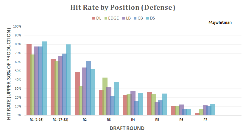
The most striking thing about this plot, as with marginalAV3, is the hit rate on Edge players in the middle of the draft. The hit rate only decreases 9% from Round 2 to Round 5, with an uptick in Round 3. The implication is not that Round 3 Edge players are better than their second round counterparts. It’s that the evaluation process is so scattershot that there isn’t much of a difference in outcomes. The second tier of the draft was not correctly identified by NFL scouts over the 14-year sample.

A potential issue at play here is over-drafting. There were 116 first-round EDGE and DL players drafted in our data set. When contrasted with the 68 OL drafted in the first over that span, it’s easy to see that there’s a premium being placed on the defensive front. The upper tier is already gone by the second round, leaving teams with plenty of room to whiff on their favorite second-tier prospect.

What We Do Now

The optimal strategy isn’t simply to draft the highest value player in each round. Teams need players at every position, not just the one that produces optimal value. So, how do we use this data to inform the draft process? Let’s take a look at a classic case.

As Eric Stoner noted last week, Anthony Chickillo is an interesting prospect, but the general thought is that he’ll go during Day 3 of the draft, right in the 4^th/5^th round sweet spot shown earlier in the MarginalAV3 plots. The problem with Chickillo is that he was used at Miami in a role very different to the one he’ll play in the NFL, and my feeling is that this phenomenon is the reason for the much of the uncertainty in DL/EDGE evaluations in general.

College teams just often don’t use EDGE and DL players correctly, and even if they’re utilized well, it’s often in roles that won’t be replicated at the next level. This means tape study leans more and more to the projection side of the spectrum and becomes less accurate.  The knowledge of this should probably change the way we interpret these prospects and their evaluations.

While the data says that there’s less value at some positions in some rounds, it doesn’t imply that there’s never value there. Antonio Brown was drafted in the 6^th round, defying the odds. Most superstar pass rushers are selected in the first round, even if the bust frequency is a little high relative to other positions.

Still, EDGE players are over-drafted, most pass-catchers are typically gone by the 4^th round, and the third round of cornerbacks are one of the worst value propositions around. This knowledge is valuable and should be incorporated into the analysis.

My recommended draft strategy would tend toward drafting offensive players in the 2^nd and 3^rd rounds while peppering the 4^th-6^th with volume picks on the defensive side of the ball. Though I don’t support strictly ruling out certain positions/round combinations, there would have to be compelling evidence toward a given prospect for me to feel comfortable drafting from a severely negative area, like 2^nd-round pass rushers, 3^rd-round corners, or 6^th-round receivers. Perhaps most importantly, I would utilize the plateaus, like 2^nd-5^th round EDGE and 2^nd-3^rd round RB, to acquire prospects with similar hit rates to peers that were drafted earlier.

The data doesn’t necessarily make us better at drafting, but it should certainly make us more cognizant of where we’ve failed in the past. Being aware of these systemic trends is the first step toward eliminating them.

–ZW

I was going to add this stat to the FAQ, but ended up with enough material that I felt it warranted a brief post. I’ve been working with a new stat: Uniqueness Index (UQI).

Similarity scores are becoming increasingly common in the draftnik world. They were originally used by Bill James to track baseball career arcs, and the same concepts can be applied to relate athletic profiles. We can use this kind of tool to compare a player from the current class to the historical NFL data set, determining a list of similar players to aid in analysis.

Uniqueness Index is a simple extension of this idea. In my simScore formulation, I define “S80” as the list of all players who achieve an 80 similarity score and above. This forms the list of all significant comparable players, with 80 representing one-half of a standard deviation from a perfect match. This is a pretty common idea with similarity scores.

I also calculate “S60,” which relates a list of players who fall, on average, within a full standard deviation of the given athletic profile. 60 represents a very weak comparison, and I don’t typically use any comps which fall below 80. Still, the players above 60 are, in a general sense, from the same category as the target profile.

UQI is simply the percentage of players in the given position group who fail to meet the S60 requirements. The basic formula is as shown below:

Players of a unique profile will have a high UQI as a smaller portion of the available data set meets the S60 similarity requirements. Standard athletic profiles will be within reach of a large portion of the available data set, and will thus have a low uniqueness.

While it’s theoretically possible to achieve a 100 UQI, the highest I have on record is 99, a mark reached by 3 of the 4 current members of the 3sigma club — Calvin Johnson, Evan Mathis, and Lane Johnson. J.J. Watt, the Fourth Musketeer, rings in at a 97.

The lower end of UQI is typically about 25-30, which represents the most dead-average profile possible. LSU OT prospect La’el Collins has one of the lower marks in the current draft class with a 27 UQI. It’s not a judgment of his ability, but does show that his build and athleticism are entirely fungible.

The correlation between UQI and SPARQ exists but is not perfect. Players who test better and worse will typically have fewer peers than those who test in the average range, but there are examples of average testers with unique profiles. For example, Wes Saxton and Jesse James are side-by-side in the TE SPARQ chart, but their UQI are very different.

The two have a nearly identical pSPARQ but fall in very different worlds of UQI. Jesse James is a more rare athlete than Wes Saxton.

That’s not necessarily good or bad. Part of the idea behind UQI is that we gain an appreciation of what we have and haven’t seen before. We can try to project Bud Dupree, but with a UQI of 95, we haven’t really seen many athletes like Bud Dupree before. To give an idea of how it works, here are a few other UQIs from the current class.:

I’ll be expanding on some further metadata related to similarity scores, but UQI is a good enough start for now.

-ZW

The idea is pretty simple: more athletic athletes are probably better at athletics than less athletic athletes. Still, it’s worth investigating any model, no matter how intuitive. Statistics also give us the benefit of determining just how much things matter, rather than the qualitative idea of “well, it probably matters.”

Before we get into the particulars, here are the different things I’ll be working with in this study:

Approximate Value – To fully investigate the impact of athleticism, it’s necessary to develop a method of assigning value to each player. As our study is intended to cover all positions, it isn’t possible to use production-based metrics, and games started aren’t necessarily a measure of value. All-Pro and Pro Bowl honors give an idea of what players are performing better, but it’s too discrete and only applies to a handful of players each year. We need something that can be applied to thousands of data points.

This is where Approximate Value comes in. Developed by Doug Drinen at Pro-Football-Reference.com, it’s a metric that gives us an integer result which represents a given player’s value for a full season. Now, AV is not perfect. I know that, and Doug knows that. This is what he wrote about it:

AV is not meant to be a be-all end-all metric. Football stat lines just do not come close to capturing all the contributions of a player the way they do in baseball and basketball. If one player is a 16 and another is a 14, we can’t be very confident that the 16AV player actually had a better season than the 14AV player. But I am pretty confident that the collection of all players with 16AV played better, as an entire group, than the collection of all players with 14AV. – Doug Drinen

The idea is that, given a large data set, Approximate Value will get things right in a broad way. With a sample size of thousands, any biases or issues with the formula wash out, leaving us with a rough idea of player value. It’s not a perfect solution, but it’s the only thing we have to conduct large, position-independent studies.

I will specifically refer to “AV3” – I’ve defined this as the sum of a given player’s three best Approximate Value seasons. This means we’re measuring peak performance. We also include the NFL betting statistics of bookmaker betting sites, as they have many data available. Others have conducted studies using the first four years of AV (i.e., the length of a rookie contract), and that’s also a valid way of expressing player value.

pSPARQ –SPARQ is a formula that measures a player’s athleticism. A higher SPARQ means a more athletic player. The specifics, inputs, etc. are all covered in other articles linked to on this site (like this one).

We then normalize pSPARQ by position. A nose tackle isn’t going to test as well as a wide receiver, so we need to somehow represent how athletic each player is by their positional average. This is possible by calculating the z-score (standard score), which is the number of standard deviations that a player’s score is above the given positional mean. Read about it on the wiki.

The idea is that we can use these standard scores and relate how athletic each player is by a single number. A 0 z-score means a player is an average NFL athlete. A z-score of 2.0 means a player is an exceptional athlete. A “3-sigma” athlete doesn’t happen very often – the NFL only has 4 current players meeting this spec.

(Those 4 players: J.J. Watt, Calvin Johnson, Evan Mathis, and Lane Johnson)

Statistical Significance – Rather than try to explain this concept, I’ll let Wikipedia do it. The main takeaway is that statistics are able to tell us the probability that a relationship exists between two variables. This all boils down to the p-value; if the p-value is 0.25, that means there is a 25% chance that the two variables are unrelated. “Significant” p-values often are smaller than 0.05, meaning there’s a  5% likelihood of no relationship (and by corollary, a 95% chance that there does exist a link). Any p-value less than 0.01 is very strong.

Weighted Least Squares Regression (WLS) – We’re working with a pretty large data set, and the scatter plot ends up being too dense to really comprehend.  The other issue is that there are a lot of zero-AVs in this data set, i.e., there are a number of players who never contributed significantly to the NFL.  This makes a scatter plot even more difficult visually because we can’t see that there are 100 scatter points stacked on top of each other at a given point.

In this kind of set, it’s common to use a weighted least squares regression, operating on the mean of the data at a list of discrete points. For our purposes, this means we would see the average AV3 of all players with a 0.2 z-score, the average AV3 of all players with a 0.3 z-score, and so on.

By operating on the mean of the data, we do not change the test for statistical significance. WLS will produce the same linear regression and strength of relationship while making it visually digestible.

With the preamble over, we can actually start regressing things.

First, let’s look at every player in the database drafted from 1999-2012. This means that we’re including 9,560 data points, drafted and undrafted. It’s probably not the best way to do things, but it’s just a starting point.

This isn’t an entirely surprising result. Undrafted players tend to be less athletic, and they just don’t succeed very often.

Note that the end of the spectrum shows data points between a z-score of 2.0 and 4.0. These look like “messy” points to the eye – there’s less of a straightforward pattern and quite a bit of scatter. This is because there are only a handful of players above 3 sigma, so averaging the data doesn’t have the smoothing effect it has in the middle of the graph, where it’s averaging hundreds of players per z-score. The scatter at the end looks odd, but we just don’t have much data there.

I won’t even bother with the statistics for the above regression as it doesn’t reflect the hypothesis we want to test. It’s probably a more relevant question to ask how this study would look if it only looked at drafted players.

I should note at this point that I am not be adjusting for draft position. This is because draft position is not causally prior to athleticism, meaning: players don’t become more athletic because they’re drafted high. They’re often drafted high due to athleticism.

We can address at a later point the relative value of athletes in different rounds, but that’s a different hypothesis. What I’m looking at in this piece is a macro-level study on if “Combine athleticism” matters. We already know it does if considering the entire group of NFL prospects. Does it matter if we restrict the sample to only the 250+ who get drafted each spring?

This looks promising, but more important is the p-value, which R reports as “< 2e-16.” This value is approximately zero, and there’s thus no chance that the relationship is just randomness. There is a statistically significant relationship between pSPARQ and Approximate Value. Yes, Combine events are able to measure the kind of athleticism that translates to NFL success.

I did some rolling averages over the end of the data to provide a little stability. Again, there are very few points from 2.0-4.0 on the x-axis, and the amount of scatter is deceptive. The following plot shows what it looks like with a little smoothing:

This is only intended to show that the data isn’t as messy as it appears. The regression is essentially the same as the first.

Note that this regression does not say that Player A with a 0 z-score is going to produce less AV than Player B with a 2.0 z-score. What it says it that a sufficiently large Group A of players that have a 0 z-score is going to produce less than those from Group B with a 2.0 z-score.

Remember that this is a starting point. It’s the most obvious regression to start with because it’s the largest. There are other, smaller studies that could be done at the positional level or with respect to draft position; however, this is a good start, and shows us that the test results we’ll see in Indianapolis do have some level of relevance.

Welcome to 3SigmaAthlete.com — I’ll be talking about SPARQ, Approximate Value, the Combine, etc., and if you’re wondering what these things are, please refer to the FAQ section of the site. I’ve tried to lay out all methodology and relevant information there.

With Combine week upon us, there will be those who feel compelled to remind the masses that football is played in pads and not underwear, fought on a gridiron and not a track. To many people, the idea that such a complex sport could be influenced by a participant’s vertical jump or short shuttle time is laughable and quickly discarded. This isn’t entirely unreasonable, as there’s too much variability inherent in the career arc of any given prospect for there to be a universally accurate projection system.

This doesn’t mean that all athleticism data should be thrown out without examination. The best approach to the draft is to look at all available data, considering information with as little bias as possible. This should never be a scouting vs. analytics issue, but rather a scouting and analytics method.

Because listing things is much easier than writing points into the natural flow of an article, here’s a list of three keys ways in which analytics can inform the scouting process.

1. Players generally won’t succeed without a certain level of athletic ability, or “functional athleticism.”

One of the biggest stumbling blocks in draft season is the comparison to an outlier. They go something along the lines of:

“Anquan Boldin ran slow at the Combine and ended up being Anquan Boldin, so Young Slow Receiver X can also have a long and successful career!”

This isn’t necessarily a criticism of these comparisons. It’s difficult to avoid the outliers because, by their nature, outliers are the data points that stick in our minds. It’s easy to remember Anquan Boldin. The problem is that there aren’t many Anquan Boldins out there.

As discussed in the FAQ on this site, the z-score stat I cite is relative to the NFL positional average. This means that a z-score of 0 refers to a player who is athletically comparable to the 50^th-percentile NFL athlete. A 0 z-score is average, a -1 z-score is below average, and a -2 z-score is a real problem.

Drawing from a database of all players drafted since 1999 and using Approximate Value (explained in the FAQ) as a rough measure of ability, there has been 1 significant guard with a z-score below -1.5. There has been 1 significant center with a z-score under -1.5. There has been 1 significant offensive tackle with a z-score less than -1.5.

For running backs, you’re looking at Reuben Droughns and Domanick Williams as the most successful sub-1.5. At corner, Brent Grimes is just about the only successful player with a z-score that falls below -1.0.

Just listing names isn’t as powerful as actual data analysis, and I’ll get to that shortly. I’m simply trying to make the case that while the outliers exist, they’re much stronger in our memories than in reality. I don’t think every offensive lineman needs to test out like Lane Johnson, but the data shows that they need to at least meet a minimum athletic requirement.

2. More athletic athletes are better athletes.

Athleticism matters. It doesn’t matter in every case, for every Boldin or Wes Welker, but it generally matters. I’ve spent the last 10 months collecting and processing data in the hope of proving this correlation statistically, and I discuss the result in a piece at great length. While I find it all fascinating, you may not be as much into the t-tests and methodology. Here’s the plot and regression that I ultimately arrived at:

If you skipped the linked article, the x-axis (horizontal axis) represents athleticism and the y-axis (vertical axis) represents NFL production. What we see is that there’s a clear trend toward more athletic players producing a higher AV3. If there was no relationship between athleticism and production, this line would be flat, parallel to the x-axis (i.e., zero slope). This relationship is statistically significant with a p-value of approximately zero.

This doesn’t mean that the more athletic player is always going to produce at a greater rate. It means that consistently picking players from a more athletic group will yield more production over the long run.

Let’s look at the first page of the wiki page on analytics.

“Analytics is the discovery and communication of meaningful patterns in data.”

The goal is to find meaningful patterns in data, often on a large scale. We aren’t able to look at 5 players and make definitive rulings on their career paths at the Combine. Over the course of time, we want to make the best value propositions with our draft capital, and you will generally find more success consistently selecting from a pool of ‘plus’ athletes than average ones.

3. Analytics should make us ask questions and re-evaluate.

Analytical athleticism comparisons can help us look back at past evaluations and question what skill or ability makes the current prospect more able to adjust to the NFL.

We don’t have Combine values for Nelson Agholor yet, but, courtesy of data maven Tony Wiltshire, I have some rough numbers he put up at his USC junior day.

Now, we don’t know that Marqise Lee won’t be a good NFL player, and he struggled through injury in his rookie season. But we know that he’s a pretty similar athlete to Agholor, will probably slot in at a similar draft position, and didn’t have an overly impressive rookie season.

In this particular case, it’s not difficult to isolate the skill that differentiates Agholor from Lee: Nelson frequently catches the ball when it’s thrown to him. The athletic comp asks how the two players are different, and we’re able to answer the question.

There’s also the case of certain athletic profiles tending to produce a high number of successful NFL players. Jordan Matthews wasn’t generally regarded as an explosive athlete last spring, but his top 4 athletic comparisons showed that he probably had the requisite athleticism to be a good NFL player. Players built like Jordan Matthews tend to do pretty well.

This doesn’t mean that he’s necessarily going to be as good as AJ Green. The intent is to look back and question the initial evaluation. Is there something that shows up on the field that contradicts the results of his athletic testing? Is there a reason to grade down his future potential on an athletic basis?

For a given prospect, the athletic profile may not tell the full story, but it’s always worth looking at the numbers and going back to the initial evaluation.

Contrary to the beliefs held by some, analytics aren’t an attempt to replace scouting or based on a belief that everything is calculable with enough spreadsheet cells. The very best NFL evaluators consistently fail. It’s a difficult job, and the hit rate isn’t great for anyone. The use of analytics is an attempt to do things more efficiently, to get incrementally better at what we’re doing.

Combine week starts tomorrow, of course, so check back in later on and I’ll have a few previews and a recap of each testing day in Indy.